Optimization story - quantum mechanics simulation speedup
Posted on
Table of Contents:
Click here for tl;dr and spoilers
I wanted to make a physics simulation 100x faster. I got it 4x faster exercising my best NumPy skills, and 50x faster after rewriting in Rust with a couple of other optimizations. After getting a machine with more (and faster) cores this jumped to 250x.
As part of my research I've been modeling absorption spectra from first principles i.e. computing how much light a protein absorbs at a given wavelength based on the locations and charges of all the atoms in the protein. Luckily, the vast majority of this work is done by collaborators running simulations on supercomputers. That process goes like this:
- Grab the structure of the protein (the precise location of all of the atoms in the protein) from the Protein Database. People spend entire careers trying to obtain these structures. I'm studying the Fenna-Matthews-Olson (FMO) complex.
- Put the protein in a box and fill the remaining space with water molecules.
- Calculate the forces between the atoms to predict where they'll move in the next time step. Apply some clever optimizations so that the simulation completes before the heat death of the universe.
- The protein structure you grabbed from the database may not be the exact structure as you'd find in nature, so let the protein jiggle around like this for a while until the atoms in the protein find equilibrium positions to jiggle around.
- Save snapshots of the protein structure during this equilibrium-jiggling for post-processing.
There's a variety of information you can extract from these snapshots, but the parts that are important to me are:
- A Hamiltonian, which is a matrix representing a quantum-mechanical description of the system and the interactions between parts of the system
- Transition dipole moments of certain molecules
- Positions of certain molecules
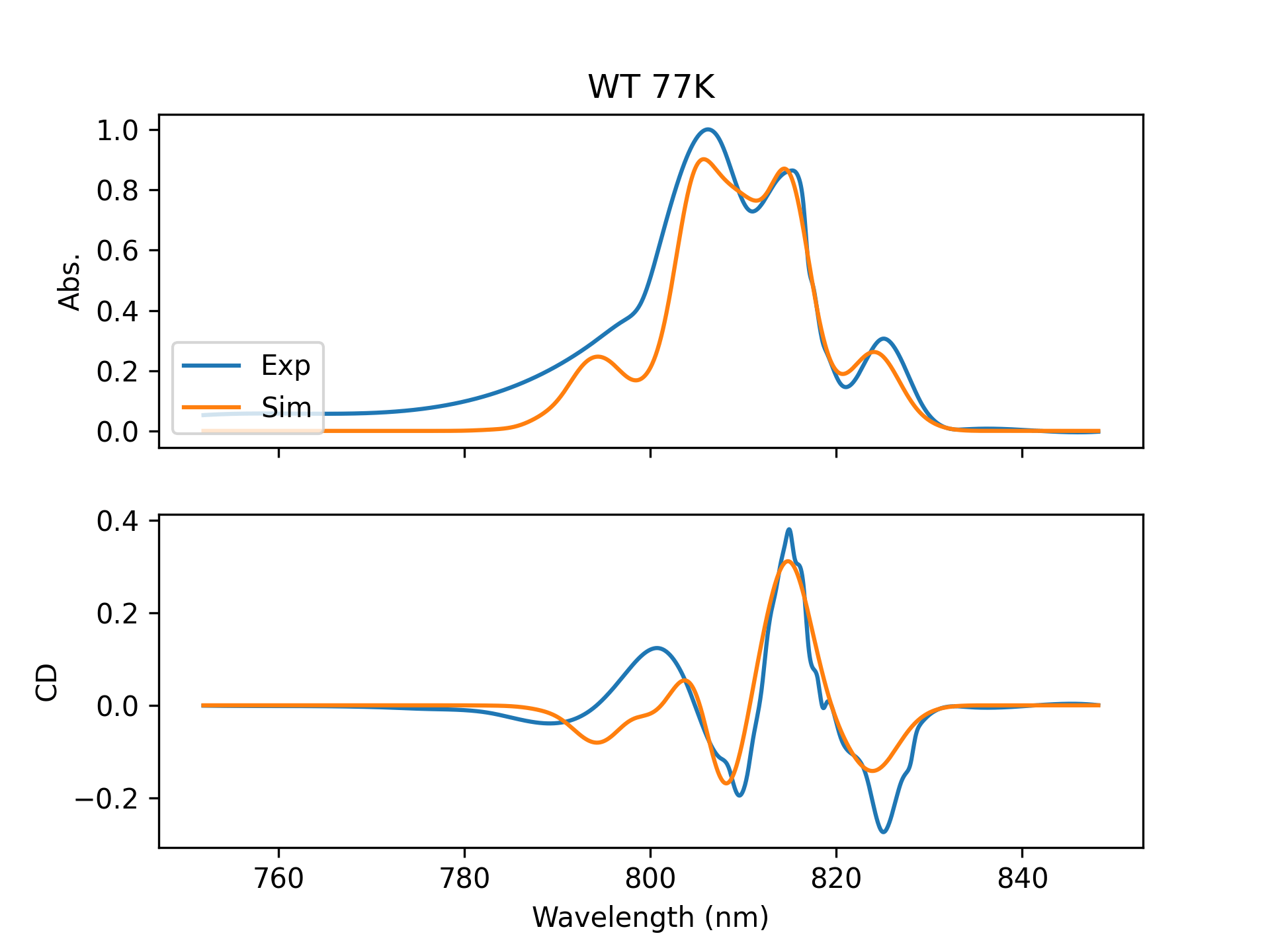
From this information I can calculate the absorption spectrum (how much light is absorbed at each wavelength) and the circular dichroism (CD) spectrum. Once I have these spectra I compare them against experimentally measured spectra to see how accurate our modeling techniques are. Sometimes it works well:
As is common in physics, part of this research entails figuring out how many details we can safely ignore. Reducing the FMO complex to an 8x8 matrix already throws away a huge number of details, namely the effect of molecular vibrations and vibrations of the entire protein, but they happen to be details that we can't calculate in a reasonable amount of time. An exact calculation would require diagonalizing a 1,000,000x1,000,000 matrix. That's an 8TB matrix (assuming 64-bit floats), and it's not a sparse one either.
Woof.
This brings us to my current task. I know that some simulations and experimental spectra don't match perfectly, so I wondered if I could fit small tweaks to the Hamiltonian (among other things) in order to get them to match. If those tweaks are within the modeling error of the simulations, that's great and it means we're on the right track. If not, it means we're leaving out important details.
Here's the problem: some fits take 8 hours to complete on my 2-core laptop. That's a hell of a feedback cycle time! The goal is to run the simulations (locally) in about 5 minutes (~100x speedup) without doing anything too crazy. We've found our rabbit hole, let's dive in!
Problem description
First let's describe the shape of my data. A complete configuration consists of:
- A Hamiltonian (8x8 array)
- The transition dipole moments (8x3 array, one row per molecule, one column each for x-, y-, and z-coordinates)
- The positions (same layout as the dipole moments).
The number of configurations used to compute the spectrum can vary. Empirically determined configurations have been published and consist of a single configuration each. The simulations our collaborators are doing produce a single configuration per snapshot, and in this case I've been supplied with 100 snapshots.
In order to calculate the absorption spectrum I first need to compute the eigenvalues and eigenvectors of the Hamiltonian (this is also called diagonalization of the Hamiltonian).
Those eigenvectors are used to compute new transition dipole moments that are weighted sums of the original dipole moments (the eigenvectors are essentially 1D arrays containing the weights). These are called "excitonic" transition dipole moments.
From these excitonic transition dipole moments I calculate the "stick spectrum" for absorption and CD. We call this a stick spectrum because it just tells you the location and magnitude (and sign, in the case of CD) of each peak in the spectrum rather than the smooth continuous curve you would normally associate with a spectrum.
From this stick spectrum we compute a "broadened" spectrum by placing a Gaussian (smooth bell curve) on top of each stick in the stick spectrum. The number of points in a broadened spectrum (the resolution) is user configurable, but in practice each one ends up being about 1500 points. If I have a single configuration, I'm done. If I have multiple configurations, I do this for each one and average them. I want to minimize the error between the computed and experimental spectra.
It's also worth going over my naming conventions. From looking at my code you'll see ham and pigs everywhere, and you may conclude from that that I have an unhealthy obsession with pork. This isn't true, in fact I'm a vegetarian. In reality ham is short for "Hamiltonian", and pigs is short for "pigments". A pigment is a light absorbing molecule (like a chlorophyll). Additionally, the mathematical symbol for a dipole moment is the Greek letter "mu", so mus is the array of dipole moments. The letter r is used to denote position, so rs is an array of positions. The snapshot files containing the Hamiltonian, dipole moments, and positions are named conf*.csv, so I call this collection of information a conf.
The code I use to run these simulations can be found here: savikhin-lab/fmo_analysis.
Finding the bottleneck
The first step in optimization is measuring to find out which part is slow. Computing spectra for multiple confs just computes individual spectra in a loop, so I decided to profile a fit of a single conf.
When it comes to Python one of my go-to tools is py-spy, a sampling profiler for Python. I ran py-spy on my fit_shifts.py script and this what it looked like:

This is the important part:
- 87.5%
make_stick_spectrum - 10%
make_broadened_spectrum
The takeaway here is that make_stick_spectrum dominates the execution time. Note that this is after I made some optimizations several weeks ago, so imagine how much more skewed towards make_stick_spectrum it would be if I had done this back then!
Aside: NumPy isn't always fast!
It turns out that NumPy's cross product function np.cross is very slow for small arrays, 10x slower than computing it manually:
m1 = np.array([1., 0., 0.])
m2 = np.array([0., 1., 0.])
# Built in, 39us
cross = np.cross(m1, m2)
# Manually, 3.9us
mu_cross = np.empty(3)
mu_cross[0] = m1[1] * m2[2] - m1[2] * m2[1]
mu_cross[1] = m1[2] * m2[0] - m1[0] * m2[2]
mu_cross[2] = m1[0] * m2[1] - m1[1] * m2[0]
This isn't a knock against NumPy. NumPy tries to work well for a wide variety of cases, provide a consistent API, provide nice error messages, etc and it generally succeeds. However, the tradeoff for all of that nice functionality appears to be significant overhead in some cases. You may be able to squeeze out some extra performance by stripping out the pieces you don't need. Another area I've done this is np.savetxt because I always know the data I'm going to save will be a certain shape.
This is what make_stick_spectrum looks like:
def make_stick_spectrum(config: Config, ham: np.ndarray, pigs: List[Pigment]) -> Dict:
    """Computes the stick spectra and eigenvalues/eigenvectors for the system."""
    ham, pigs = delete_pigment(config, ham, pigs)
    n_pigs = ham.shape[0]
    if config.delete_pig > n_pigs:
        raise ValueError(f"Tried to delete pigment {config.delete_pig} but system only has {n_pigs} pigments.")
    e_vals, e_vecs = np.linalg.eig(ham)
    pig_mus = np.zeros((n_pigs, 3))
    if config.normalize:
        total_dpm = np.sum([np.dot(p.mu, p.mu) for p in pigs])
        for i in range(len(pigs)):
            pigs[i].mu /= total_dpm
    for i, p in enumerate(pigs):
        pig_mus[i, :] = pigs[i].mu
    exciton_mus = np.zeros_like(pig_mus)
    stick_abs = np.zeros(n_pigs)
    stick_cd = np.zeros(n_pigs)
    for i in range(n_pigs):
        exciton_mus[i, :] = np.sum(np.repeat(e_vecs[:, i], 3).reshape((n_pigs, 3)) * pig_mus, axis=0)
        stick_abs[i] = np.dot(exciton_mus[i], exciton_mus[i])
        energy = e_vals[i]
        if energy == 0:
            # If the energy is zero, the pigment has been deleted
            # so put it somewhere far away to avoid dividing by zero
            energy = 100_000
        wavelength = 1e8 / energy  # in angstroms
        stick_coeff = 2 * np.pi / wavelength
        for j in range(n_pigs):
            for k in range(n_pigs):
                r = pigs[j].pos - pigs[k].pos
                # NumPy cross product function is super slow for small arrays
                # so we do it by hand for >10x speedup.
                mu_cross = np.empty(3)
                mu_cross[0] = pigs[j].mu[1] * pigs[k].mu[2] - pigs[j].mu[2] * pigs[k].mu[1]
                mu_cross[1] = pigs[j].mu[2] * pigs[k].mu[0] - pigs[j].mu[0] * pigs[k].mu[2]
                mu_cross[2] = pigs[j].mu[0] * pigs[k].mu[1] - pigs[j].mu[1] * pigs[k].mu[0]
                stick_cd[i] += e_vecs[j, i] * e_vecs[k, i] * np.dot(r, mu_cross)
        stick_cd[i] *= stick_coeff
    out = {
        "ham_deleted": ham,
        "pigs_deleted": pigs,
        "e_vals": e_vals,
        "e_vecs": e_vecs,
        "exciton_mus": exciton_mus,
        "stick_abs": stick_abs,
        "stick_cd": stick_cd
    }
    return out
Even to my eyes it's not immediately obvious where the bottleneck would be in this function. In order to continue looking for the bottleneck we'll use another tool: line_profiler. A flamegraph tells you which function is slow, but not necessarily what about it is slow. line_profiler annotates each line with information about its execution time so you can immediately see where the time is going. Running line_profiler on make_stick_spectrum generates this report:
Click here to expand the report
Timer unit: 1e-06 s

Total time: 0.010513 s
File: /Users/zmitchell/code/research/fmo_analysis/fmo_analysis/exciton.py
Function: make_stick_spectrum at line 37

Line #      Hits         Time  Per Hit   % Time  Line Contents
==============================================================
    37                                           def make_stick_spectrum(config: Config, ham: np.ndarray, pigs: List[Pigment]) -> Dict:
    38                                               """Computes the stick spectra and eigenvalues/eigenvectors for the system."""
    39         1          8.0      8.0      0.1      ham, pigs = delete_pigment(config, ham, pigs)
    40         1          2.0      2.0      0.0      n_pigs = ham.shape[0]
    41         1          4.0      4.0      0.0      if config.delete_pig > n_pigs:
    42                                                   raise ValueError(f"Tried to delete pigment {config.delete_pig} but system only has {n_pigs} pigments.")
    43         1        768.0    768.0      7.3      e_vals, e_vecs = np.linalg.eig(ham)
    44         1         32.0     32.0      0.3      pig_mus = np.zeros((n_pigs, 3))
    45         1          5.0      5.0      0.0      if config.normalize:
    46                                                   total_dpm = np.sum([np.dot(p.mu, p.mu) for p in pigs])
    47                                                   for i in range(len(pigs)):
    48                                                       pigs[i].mu /= total_dpm
    49         8         36.0      4.5      0.3      for i, p in enumerate(pigs):
    50         7         63.0      9.0      0.6          pig_mus[i, :] = pigs[i].mu
    51         1         46.0     46.0      0.4      exciton_mus = np.zeros_like(pig_mus)
    52         1          3.0      3.0      0.0      stick_abs = np.zeros(n_pigs)
    53         1          3.0      3.0      0.0      stick_cd = np.zeros(n_pigs)
    54         8         12.0      1.5      0.1      for i in range(n_pigs):
    55         7        478.0     68.3      4.5          exciton_mus[i, :] = np.sum(np.repeat(e_vecs[:, i], 3).reshape((n_pigs, 3)) * pig_mus, axis=0)
    56         7         84.0     12.0      0.8          stick_abs[i] = np.dot(exciton_mus[i], exciton_mus[i])
    57         7         10.0      1.4      0.1          energy = e_vals[i]
    58         7         23.0      3.3      0.2          if energy == 0:
    59                                                       # If the energy is zero, the pigment has been deleted
    60                                                       energy = 100_000
    61         7         14.0      2.0      0.1          wavelength = 1e8 / energy  # in angstroms
    62         7         15.0      2.1      0.1          stick_coeff = 2 * np.pi / wavelength
    63        56        102.0      1.8      1.0          for j in range(n_pigs):
    64       392        689.0      1.8      6.6              for k in range(n_pigs):
    65       343       1167.0      3.4     11.1                  r = pigs[j].pos - pigs[k].pos
    66                                                           # NumPy cross product function is super slow for small arrays
    67                                                           # so we do it by hand for >10x speedup. It makes a difference!
    68       343       1112.0      3.2     10.6                  mu_cross = np.empty(3)
    69       343       1230.0      3.6     11.7                  mu_cross[0] = pigs[j].mu[1] * pigs[k].mu[2] - pigs[j].mu[2] * pigs[k].mu[1]
    70       343        953.0      2.8      9.1                  mu_cross[1] = pigs[j].mu[2] * pigs[k].mu[0] - pigs[j].mu[0] * pigs[k].mu[2]
    71       343       1020.0      3.0      9.7                  mu_cross[2] = pigs[j].mu[0] * pigs[k].mu[1] - pigs[j].mu[1] * pigs[k].mu[0]
    72       343       2611.0      7.6     24.8                  stick_cd[i] += e_vecs[j, i] * e_vecs[k, i] * np.dot(r, mu_cross)
    73         7         11.0      1.6      0.1          stick_cd[i] *= stick_coeff
    74         1          3.0      3.0      0.0      out = {
    75         1          1.0      1.0      0.0          "ham_deleted": ham,
    76         1          1.0      1.0      0.0          "pigs_deleted": pigs,
    77         1          1.0      1.0      0.0          "e_vals": e_vals,
    78         1          1.0      1.0      0.0          "e_vecs": e_vecs,
    79         1          1.0      1.0      0.0          "exciton_mus": exciton_mus,
    80         1          2.0      2.0      0.0          "stick_abs": stick_abs,
    81         1          1.0      1.0      0.0          "stick_cd": stick_cd
    82                                               }
    83         1          1.0      1.0      0.0      return out
This is what we learn from the report:
- 7.3% diagonalizing the Hamiltonian (line 43)
- 4.5% computing exciton dipole moments (line 55)
- 0.8% computing stick absorption (line 56)
- 77% computing stick CD (lines 65-72)
So, let's focus on computing CD!
Optimizing CD
At this point I decided to make myself some tools. I made a script for running line_profiler and a script for timing the execution of a single function, then checked both of these into git so that I can reuse them at a later date without needing to reinvent the wheel.
My execution timing script boils down to this:
from time import perf_counter
from fmo_analysis import exciton


def main():
    ham, pigs = ...
    n = 10_000
    times = []
    for _ in range(n):
        t_start = perf_counter()
        stick = exciton.make_stick_spectrum(config, ham, pigs)
        t_stop = perf_counter()
        times.append(t_stop - t_start)
    per_call = sum(times) / n * 1e3
    print(f"{per_call:.4f}ms per call")


if __name__ == "__main__":
    main()
The execution time varies from moment to moment depending on what else is running on my laptop, what's in cache, etc so the exact times should be taken with a grain of salt. Our starting point is 3.48ms per call to make_stick_spectrum.
Avoiding superfluous lookups
The first thing that jumped out at me is that we're repeatedly looking up the two pigments pigs[j] and pigs[k] in the inner loop. Looking these pigments up once at the beginning of the loop e.g. pig_j = pigs[j] takes us from 3.48ms to 2.78ms for a 25% speedup.
The CD calculation now looks like this for a single "stick":
for j in range(n_pigs):
    for k in range(n_pigs):
        pig_j = pigs[j]
        pig_k = pigs[k]
        r = pig_j.pos - pig_k.pos
        # NumPy cross product function is super slow for small arrays
        # so we do it by hand for >10x speedup.
        mu_cross = np.empty(3)
        mu_j = pig_j.mu
        mu_k = pig_k.mu
        mu_cross[0] = mu_j[1] * mu_k[2] - mu_j[2] * mu_k[1]
        mu_cross[1] = mu_j[2] * mu_k[0] - mu_j[0] * mu_k[2]
        mu_cross[2] = mu_j[0] * mu_k[1] - mu_j[1] * mu_k[0]
        # Calculate the dot product by hand, 2x faster than np.dot()
        r_mu_dot = r[0] * mu_cross[0] + r[1] * mu_cross[1] + r[2] * mu_cross[2]
        stick_cd[i] += e_vecs[j, i] * e_vecs[k, i] * r_mu_dot
Skipping half of the calculations
It turns out that the computation for a pair of pigments j and k is identical to the computation for k and j. Put another way, if you swap j and k nothing changes. Swapping r_j and r_k gives you a minus sign. Swapping mu_j and mu_k also gives you a minus sign. These two minus signs cancel out when you calculate (r_j - r_k) * (mu_j x mu_k). This means we only need to calculate the CD contribution for each pair of pigments once and then double it (i.e. 2 * cd(j,k)) rather than calculating it separately for j,k and k,j (i.e. cd(j,k) + cd(k,j)).
for j in range(n_pigs):
    for k in range(j, n_pigs):  # Notice the "j" here now!
        ...
        # Notice the "2" here now!
        stick_cd[i] += 2 * e_vecs[j, i] * e_vecs[k, i] * r_mu_dot
This takes us from 2.78ms to 1.71ms for a 63% speedup.
Skipping the diagonal
The key calculation is this (r_j - r_k) * (mu_j x mu_k) piece. Both (r_j - r_k) and (mu_j x mu_k) are zero if j = k, so we can skip those calculations entirely. This is all we need to change:
for j in range(n_pigs):
    for k in range(j+1, n_pigs):  # Notice the "+1" here!
This takes us from 1.71ms to 1.41ms for an 21% speedup.
Caching some computations
If you look at the (r_j - r_k) * (mu_j x mu_k) piece, you'll notice a distinct lack of i. This means we're calculating it over and over again for no reason on every iteration of the outer loop. We can calculate this part once and reuse it. The outer loop looks like this now:
r_mu_cross_cache = make_r_dot_mu_cross_cache(pigs)
for i in range(n_pigs):
    exciton_mus[i, :] = np.sum(np.repeat(e_vecs[:, i], 3).reshape((n_pigs, 3)) * pig_mus, axis=0)
    stick_abs[i] = np.dot(exciton_mus[i], exciton_mus[i])
    energy = e_vals[i]
    if energy == 0:
        # If the energy is zero, the pigment has been deleted
        energy = 100_000
    wavelength = 1e8 / energy  # in angstroms
    stick_coeff = 2 * np.pi / wavelength
    e_vec_weights = make_weight_matrix(e_vecs, i)
    stick_cd[i] = 2 * stick_coeff * np.sum(e_vec_weights * r_mu_cross_cache)
where make_r_mu_cross_cache and make_weight_matrix look like this:
def make_r_dot_mu_cross_cache(pigs):
    """Computes a cache of (r_i - r_j) * (mu_i x mu_j)"""
    n = len(pigs)
    cache = np.zeros((n, n))
    for i in range(n):
        for j in range(i+1, n):
            r_i = pigs[i].pos
            r_j = pigs[j].pos
            r_ij = r_i - r_j
            mu_i = pigs[i].mu
            mu_j = pigs[j].mu
            mu_ij_cross = np.empty(3)
            mu_ij_cross[0] = mu_i[1] * mu_j[2] - mu_i[2] * mu_j[1]
            mu_ij_cross[1] = mu_i[2] * mu_j[0] - mu_i[0] * mu_j[2]
            mu_ij_cross[2] = mu_i[0] * mu_j[1] - mu_i[1] * mu_j[0]
            cache[i, j] = r_ij[0] * mu_ij_cross[0] + r_ij[1] * mu_ij_cross[1] + r_ij[2] * mu_ij_cross[2]
    return cache


def make_weight_matrix(e_vecs, col):
    """Makes the matrix of weights for CD from the eigenvectors"""
    n = e_vecs.shape[0]
    mat = np.zeros((n, n))
    for i in range(n):
        for j in range(i+1, n):
            mat[i, j] = e_vecs[i, col] * e_vecs[j, col]
    return mat
This takes us from 1.41ms to 0.94ms for a 50% speedup.
Letting NumPy take control
The more you can keep execution in C and out of Python, the faster your program is going to run. In practice this means letting NumPy do iteration for you and apply functions to entire arrays since it can iterate and apply functions in C, which is much faster. Consider this example: I want to multiply two matrices together elementwise and sum the result.
The naive version looks like this:
np.sum(e_vec_weights * r_mu_cross_cache)
The product here creates a new array containing the product, and np.sum adds the elements of that new matrix.
There's another operation similar to this called the "dot product" or "inner product", but in order to get a single number out of it you need two 1D arrays. Luckily there's a built-in method, flatten, which converts a multi-dimensional array into a 1D array. Since these two matrices are the same shape I know they'll be flattened such that corresponding elements line up properly for the dot product:
np.dot(e_vec_weights.flatten(), r_mu_cross_cache.flatten())
This is roughly 3x faster than the naive method. It's not a big speedup overall in this program (0.94ms to 0.91ms for a 3% speedup) but it's instructive anyway.
Calling LAPACK routines directly
At this point the breakdown of execution time looks like this:
- 50% computing eigenvalues and eigenvectors
- 16% making the cache
- 9% making the weights to go along with the cache
- 10% computing the exciton dipole moments
Calculating CD no longer dominates the execution time, so I moved my focus to diagonalization. I knew that my Hamiltonian matrix was symmetric, so I wondered if there were diagonalization algorithms that could take advantage of this. Fortunately NumPy has one built in: eigh. Unfortunately it didn't seem to make much of a difference (within measurement error on my laptop). I suspect that there may be a bigger difference on a larger matrix.
I wondered again whether NumPy was adding some overhead. One of the things that makes NumPy so fast is that parts of it are wrappers around LAPACK and BLAS, which are industry standard libraries for efficient linear algebra algorithms and operations. In order to test out this hypothesis I decided to call the LAPACK diagonalization routine directly as made available by the scipy.lapack module. The LAPACK routine used by eig is called DGEEV. Yeah, it's cryptic.
A tricky detail here is that LAPACK is written in FORTRAN, so it expects and returns arrays with FORTRAN-ordering (column-major) rather than C-ordering (row-major), so you need to handle conversion between the two. Fortunately my Hamiltonian is symmetric so the FORTRAN ordering is actually identical to the C-ordering. This isn't the case for the return values, though.
This is what the new diagonalization code looks like:
e_vals_fortran_order, _, _, e_vecs_fortran_order, _ = lapack.sgeev(ham)
e_vals = np.ascontiguousarray(e_vals_fortran_order)
e_vecs = np.ascontiguousarray(e_vecs_fortran_order)
This takes us from 0.91ms to 0.85ms for a 7% speedup.
At this point we've managed to reduce the execution time from 3.48ms to 0.85ms for a 4x speedup. The goal is 100x, so we're missing our target by 25x. That's a lot of x's and I'm running out of NumPy tricks. It's time to call in the big guns.
Rust rewrite
I know it's a meme at this point, but I decided to rewrite the number-crunching parts of this program in Rust. There are four crates that make this possible:
- PyO3, for Rust/Python interop
- maturin, for interacting with your extension during development and eventually publishing it to PyPI
- ndarray, Rust's equivalent to NumPy
- rust-numpy, for converting between NumPy and ndarray
The Python interop was shockingly easy. I wouldn't even know how to begin doing this with C. It's not without friction, but that's mostly a documentation issue. For instance, I had trouble putting my Rust source alongside my Python source in my Python package and having poetry build include the compiled Rust binary. The documentation makes it sound like this is the preferred method, but I couldn't figure it out in the moment and I was short on time. It's entirely possible I missed something simple, I've never done this before.
I ended up just making a separate package, ham2spec, so I could upload it to PyPI and have it downloaded and installed like any other dependency. I shouldn't have to build and upload my Rust extension to a server somewhere to get it picked up properly as a dependency of my local project, but here we are.
This is what the development process looks like:
- Create a new project with
maturin new - Write your Rust code
- Package it up and expose it to Python locally with
maturin develop - Fire up a Python interpreter and play around with your module to give things a cursory glance
- Repeat
- Publish your module with
maturin publish
I also decided to interface with LAPACK directly via the lapack crate. I have one use of unsafe in my crate and it's the call to dgeev. I'm ok with that.
The Rust code is a pretty direct translation from the Python code. I had an inkling from the beginning that I would need to write the number crunching code in Rust, but it was easier to explore optimizations in Python first. The only real deviations are the use of all the nice iterators that Rust provides, especially the Zip iterator that ndarray provides for iterating over multiple arrays in lock-step. Here's Zip in action:
pub fn compute_stick_spectra(
    hams: ArrayView3<f64>,
    mus: ArrayView3<f64>,
    rs: ArrayView3<f64>,
) -> Vec<StickSpectrum> {
    let dummy_stick = StickSpectrum {
        e_vals: arr1(&[]),
        e_vecs: arr2(&[[], []]),
        mus: arr2(&[[], []]),
        stick_abs: arr1(&[]),
        stick_cd: arr1(&[]),
    };
    let mut sticks: Vec<StickSpectrum> = Vec::with_capacity(hams.dim().0);
    sticks.resize(hams.dim().0, dummy_stick);
    Zip::from(hams.axis_iter(Axis(0)))
        .and(mus.axis_iter(Axis(0)))
        .and(rs.axis_iter(Axis(0)))
        .and(&mut sticks)
        .for_each(|h, m, r, s| *s = compute_stick_spectrum(h, m, r));
    sticks
}
This direct translation executes in 35us for a total speedup of ~100x, but there's a bit of a catch. The Rust code takes 3 arrays as arguments (8x8 Hamiltonian, 8x3 dipole moments, 8x3 positions), whereas the previous Python function is called with an 8x8 array for the Hamiltonian and a list of Pigment objects, which are each just containers for a position and a dipole moment. Doing the conversion to arrays brings the execution time to 45us. I'm still counting this as a win since I don't have to do this conversion, I'm just doing it to preserve backwards compatibility with a bunch of simulations I've already written.
Just for kicks I decided to profile ham2spec to see if there was any low-hanging fruit for optimization. In order to do this I had to create a crate example since my crate is a library, not a binary, and examples get compiled into their own binaries. I made this example and profiled it with cargo-flamegraph. The profiling output showed that the runtime of compute_stick_spectrum (my Rust equivalent of the make_stick_spectrum function from my Python code) looked like this:
- 45% diagonalization
- 23% computing exciton dipole moments
- 24% computing CD
If I could somehow magically eliminate my own calculations entirely and let diagonalization dominate the execution time I would only make this function ~2x faster. I already know that we've eliminated the stick spectrum bottleneck, so this isn't worth it.
The only thing left to do is make sure the output of the new code and old code match up...
Matching outputs
It's at this point that I must make a confession. I haven't been eating my vegetables. Well, I have, like I said I'm a vegetarian. What I really mean is that I didn't have a test suite for either fmo_analysis or ham2spec. I know, blasphemy.
I'm the last person you need to convince about writing tests. I've given talks about esoteric testing techniques. I've also written about the need for better testing in scientific software and property-based testing specifically. So, how did we get here?
- Burnout. Graduate school is hard. Doing anything that doesn't directly move you towards graduation has a high activation energy.
- I'm the only person on the planet using this software, so I'll just run into all the bugs myself and fix them. Right?
- This started as a small CLI that I threw together and it quickly grew beyond that scope.
- My dog ate my test suite.
Suffice to say that I now have test suites for both fmo_analysis and ham2spec.
The problem was multi-faceted:
- I wasn't converting between memory orderings correctly
- Eigenvectors are only defined up to a sign, so small differences in precision can cause sign flips
- I had switched from double-precision to single-precision, which caused sign flips as mentioned above
- The allegedly "known-good" data I was comparing against was saved incorrectly (when in doubt, test the test!)
Ultimately the sign flips don't change the results, but I had to change my test suite to allow for sign flips.
Aside: Converting between orderings
An n-dimensional array in NumPy or ndarray consists of a few pieces of information:
- The buffer containing the actual data
- The dimensions of the array
- The strides, or "how many elements do I have to traverse in the buffer to get to the next item along a particular axis"
You can see that here in ndarray and here in NumPy.
When you ask for the transpose of an array (swapping the rows and columns) it's these dimensions and strides that are modified, not the underlying data. For instance, this is how ndarray::ArrayBase::reversed_axes is implemented:
/// Transpose the array by reversing axes.
///
/// Transposition reverses the order of the axes (dimensions and strides)
/// while retaining the same data.
pub fn reversed_axes(mut self) -> ArrayBase<S, D> {
    self.dim.slice_mut().reverse();
    self.strides.slice_mut().reverse();
    self
}
This is a good idea because the data structures for dimensions and strides are small and quickly modified. Copying the contents of the array into a new array in a different order is much slower. In order to actually transpose the data in the buffer you have to do this:
let transposed = my_arr
    .reversed_axes()
    .as_standard_layout()  // Returns a CowArray (Cow = copy-on-write)
    .to_owned();  // Necessary to get an owned array
Broadened spectra
Once everything was correct, I got back to work optimizing. My stick spectrum computations were 100x faster, so it was time to look at how that translated to computing a broadened spectrum. As a refresher, computing a broadened spectrum looks like this:
- Compute the stick spectrum from a Hamiltonian
- Compute a broadened spectrum from a stick spectrum
I timed the execution of the original system computing a spectrum from 100 Hamiltonians and it took 381ms. It's no wonder that a fit takes forever when each iteration of the minimization routine takes almost 400ms.
I timed the execution of the new system doing the same computation and it took 40ms. That's only 10x faster! My stick spectrum computations were 100x faster than the old version, so why is this so much slower? As a reminder, this was the original breakdown of execution time:
- 87.5%
make_stick_spectrum - 10%
make_broadened_spectrum
If you magically eliminate the runtime of everything but make_broadened_spectrum you would only expect a 10x speedup (100% -> 10%).
We effectively did elminate the execution time of everything else, so we're seeing exactly that 10x speedup we would expect. So, how do we make it faster?
Making it parallel
The process of computing a broadened spectrum from each Hamiltonian falls into the category of embarrassingly parallel, so we don't even need to do much work to make this parallel. I literally changed a for_each to a par_for_each:
Zip::from(abs_arr.columns_mut())
    .and(cd_arr.columns_mut())
    .and(hams.axis_iter(Axis(0)))
    .and(mus.axis_iter(Axis(0)))
    .and(rs.axis_iter(Axis(0)))
    .par_for_each(|mut abs_col, mut cd_col, h, m, r| { // <-- parallel iteration here!
        let stick = compute_stick_spectrum(h, m, r);
        let broadened = compute_broadened_spectrum_from_stick(
            stick.e_vals.view(),
            stick.stick_abs.view(),
            stick.stick_cd.view(),
            config,
        );
        abs_col.assign(&broadened.abs);
        cd_col.assign(&broadened.cd);
    });
}
This brought the execution time from 40ms to 17.6ms for a 127% speedup. My puny laptop only has 2 cores (but it does have Hyper-threading), so this is in the ballpark of what I would expect. I do have a new 16" Macbook Pro on the way with many more cores to throw at this, so we'll see if I get linear scaling with the number of cores or not.
At this point we're still only 22x faster than the original execution time of 381ms for computing a broadened spectrum from 100 Hamiltonians.
Doing less work
I ran cargo-flamegraph on an example calculation and it showed that calls to exp account for 55% of the execution time. On one hand, that's not a function I can make faster by modifying its code, so that's discouraging. On the other hand it means that most of the execution time is spent doing calculations and nothing too weird.
I remember reading a post or a comment somewhere from Andrew Gallant, the original brain behind ripgrep, that said something along the lines of "one of the easiest ways to make a program faster is to make it do less work." That's always stuck with me. How does it apply here?
We're placing a Gaussian on top of each stick in the stick spectrum, but the contribution from each Gaussian diminishes as you get further away from the peak. If you get far enough away from the peak, the contributions become vanishingly small. If that's the case, why do those calculations at all?
I decided that instead of computing each Gaussian for all x-values in the domain I would only compute each Gaussian within a user-configurable range of the peak.
/// Determine the indices for which you actually need to compute the contribution of a band
pub fn band_cutoff_indices(center: f64, bw: f64, cutoff: f64, xs: &[f64]) -> (usize, usize) {
    let lower = xs.partition_point(|&x| x < (center - cutoff * bw));
    let upper = xs.partition_point(|&x| x < (center + cutoff * bw));
    (lower, upper)
}

/// Computes the band and adds it to the spectrum
pub fn add_cutoff_bands(
    mut spec: ArrayViewMut1<f64>,
    energies: ArrayView1<f64>,
    stick_strengths: ArrayView1<f64>,
    bws: &[f64],
    cutoff: f64,
    x: ArrayView1<f64>,
) {
    Zip::from(energies)
        .and(stick_strengths)
        .and(bws)
        .for_each(|&e, &strength, &bw| {
            let denom = gauss_denom(bw);
            let (lower, upper) = band_cutoff_indices(e, bw, cutoff, x.as_slice().unwrap());
            let band = x
                .slice(s![lower..upper])
                .mapv(|x_i| strength * (-(x_i - e).powi(2) / denom).exp());
            spec.slice_mut(s![lower..upper]).add_assign(&band);
        });
}
This takes us from 17.6ms to 8.1ms with a cutoff of 3 for a 117% speedup. Now we're sitting at 47x faster than the original.
Final attempts
At this point I was running out of low-hanging fruit and turned to some heavier-duty tools and shots in the dark.
Looking at the assembly
I used cargo-asm to view the assembly (compiled with --release) of add_cutoff_bands:
ham2spec::add_cutoff_bands (src/lib.rs:337):
 push    rbp
 mov     rbp, rsp
 push    r14
 push    rbx
 sub     rsp, 64
 movsd   qword, ptr, [rbp, -, 24], xmm0
 mov     rax, qword, ptr, [rsi, +, 8]
 cmp     qword, ptr, [rdx, +, 8], rax
 jne     LBB44_7
 cmp     rax, r8
 jne     LBB44_7
 mov     r10, rdi
 mov     r14, qword, ptr, [rsi]
 mov     rsi, qword, ptr, [rsi, +, 16]
 mov     r11, qword, ptr, [rdx]
 mov     rdi, qword, ptr, [rdx, +, 16]
 cmp     rsi, 1
 sete    dl
 cmp     r8, 2
 setb    al
 or      dl, al
 cmp     rdi, 1
 sete    bl
 cmp     dl, 1
 jne     LBB44_4
 or      bl, al
 je      LBB44_4
 mov     qword, ptr, [rbp, -, 48], r14
 mov     qword, ptr, [rbp, -, 40], r11
 mov     qword, ptr, [rbp, -, 32], rcx
 movaps  xmm0, xmmword, ptr, [rip, +, LCPI44_0]
 movaps  xmmword, ptr, [rbp, -, 80], xmm0
 jmp     LBB44_6
LBB44_4:
 mov     qword, ptr, [rbp, -, 48], r14
 mov     qword, ptr, [rbp, -, 40], r11
 mov     qword, ptr, [rbp, -, 32], rcx
 mov     qword, ptr, [rbp, -, 80], rsi
 mov     qword, ptr, [rbp, -, 72], rdi
LBB44_6:
 mov     qword, ptr, [rbp, -, 64], 1
 lea     rdi, [rbp, -, 48]
 lea     rsi, [rbp, -, 80]
 lea     rcx, [rbp, -, 24]
 mov     rdx, r8
 mov     r8, r9
 mov     r9, r10
 call    ndarray::zip::Zip<P,D>::inner
 add     rsp, 64
 pop     rbx
 pop     r14
 pop     rbp
 ret
LBB44_7:
 lea     rdi, [rip, +, l___unnamed_37]
 lea     rdx, [rip, +, l___unnamed_38]
 mov     esi, 43
 call    core::panicking::panic
Well, all of the interesting stuff (the call to for_each) happens inside the call to ndarray::zip::Zip<P, D>::inner and I don't know how to get at that with cargo asm. I fired up a debugger and disassembled add_cutoff_bands, but this left me with the opposite problem (a sea of assembly). I wasn't able to glean much from this just because I can barely read assembly. Sorry.
I was looking for signs one way or the other whether the computations were being vectorized. It's still unclear to me whether that's happening.
Instruction level parallelism
I recently read a series of posts showing how a Rust program was progressively optimized and made to run in parallel (Comparing Parallel Rust and C++) and one of the optimizations seemed relatively easy: loop unrolling.
I decided to give it a try by operating on chunks of data at a time, like this:
/// The block size for doing chunked computations
const BLOCK_SIZE: usize = 4;

/// Compute the band cutoff indices aligned to the block size
fn block_aligned_band_cutoff_indices(
    bsize: usize,
    center: f64,
    bw: f64,
    cutoff: f64,
    xs: &[f64],
) -> (usize, usize) {
    let lower = xs.partition_point(|&x| x < (center - cutoff * bw));
    let upper = xs.partition_point(|&x| x < (center + cutoff * bw));
    let rem = (upper - lower) % bsize;
    // The higher energy side tends to have less going on, so we can err
    // on the side of computing fewer values there
    return (lower, upper - rem);
}

/// Compute the cutoff bands using SIMD
fn add_cutoff_bands_chunked(
    mut spec: ArrayViewMut1<f64>,
    energies: ArrayView1<f64>,
    stick_strengths: ArrayView1<f64>,
    bws: &[f64],
    cutoff: f64,
    x: ArrayView1<f64>,
) {
    let band_indices: Vec<(usize, usize)> = energies
        .iter()
        .zip(bws.iter())
        .map(|(&e, &b)| {
            block_aligned_band_cutoff_indices(BLOCK_SIZE, e, b, cutoff, x.as_slice().unwrap())
        })
        .collect();
    let denoms: Vec<f64> = bws.iter().map(|&b| gauss_denom(b)).collect();
    let x_slice = x.as_slice().unwrap();
    let spec_slice = spec.as_slice_mut().unwrap();
    for (&e, (&s, (&d, bi))) in energies
        .iter()
        .zip(stick_strengths.iter().zip(denoms.iter().zip(band_indices)))
    {
        x_slice[bi.0..bi.1]
            .chunks_exact(BLOCK_SIZE)
            .zip(spec_slice.chunks_exact_mut(BLOCK_SIZE))
            .for_each(|(x_chunk, s_chunk)| {
                s_chunk[0] += s * (-(x_chunk[0] - e).powi(2) / d).exp();
                s_chunk[1] += s * (-(x_chunk[1] - e).powi(2) / d).exp();
                s_chunk[2] += s * (-(x_chunk[2] - e).powi(2) / d).exp();
                s_chunk[3] += s * (-(x_chunk[3] - e).powi(2) / d).exp();
            });
    }
}
This was actually marginally slower, 8.4ms vs. 8.1ms. However, it's very clear from the assembly that the operations are being vectorized. Here's a snippet where it's clear that actual math is being done:
LBB44_100:
 movupd  xmm1, xmmword, ptr, [r14, +, 8*rdi]
 mulpd   xmm1, xmm1
 divpd   xmm1, xmm0
 movupd  xmmword, ptr, [rbx, +, 8*rdi], xmm1
 movupd  xmm1, xmmword, ptr, [r14, +, 8*rdi, +, 16]
 mulpd   xmm1, xmm1
 divpd   xmm1, xmm0
 movupd  xmmword, ptr, [rbx, +, 8*rdi, +, 16], xmm1
 add     rdi, 4
 add     rsi, 2
 jne     LBB44_100
 test    dl, 1
 je      LBB44_103
LBB44_102:
 movupd  xmm0, xmmword, ptr, [r14, +, 8*rdi]
 mulpd   xmm0, xmm0
 divpd   xmm0, xmmword, ptr, [rip, +, LCPI44_0]
 movupd  xmmword, ptr, [rbx, +, 8*rdi], xmm0
Unfortunately, I don't have much insight into why this is slower. If I had to guess, I would say that it's a combination of the following:
- My laptop only has 128-bit floating point SIMD registers, so you're only operating on two
f64s at a time - SIMD instructions have significantly higher latency than scalar instructions
Perhaps the SIMD overhead outweighs the (at best) 2x speedup from using SIMD instructions?
Explicit SIMD
Just for kicks I decided to try writing the SIMD code myself rather than relying on the compiler to do it for me. It's worth noting that it's not very clear to me what the current recommendation is when it comes to SIMD crates. These are the official options:
- The std::simd module, only available with the Nightly compiler
- Architecture specific implementations in the
std::archmodule, which comes from the stdarch crate - The packed_simd crate
In the end I decided to go with packed_simd because it looked the most ergonomic. It only took a slight modification of the chunked code to get it working with SIMD.
This brought execution time from 8.1ms to 7.4ms for a 9% speedup (51x overall).
I decided not to keep this implementation because it requires a Nightly compiler and it would require supporting different architectures (I have an Apple Silicon laptop on the way).
Cachegrind
I wondered if there was anything egregiously cache-inefficient, so I decided to try running a program under Cachegrind. Cachegrind essentially doesn't support macOS so I put together a Docker container for doing this analysis:
FROM rust:latest

# Install build-time dependencies, remove cruft afterwards
RUN apt-get update && apt-get install -y valgrind libopenblas-dev gfortran python3 python3-pip && rm -rf /var/lib/apt/lists/*
RUN python3 -m pip install --user numpy

# Cache the Rust dependencies so they don't download on every recompile
WORKDIR /ham2spec
COPY Cargo.toml .
RUN mkdir src && touch src/lib.rs && cargo vendor

# Copy the code over
COPY src/ ./src/
COPY examples/ ./examples/

# Compile the example
RUN RUSTFLAGS='-C force-frame-pointers=y' cargo build --example multiple_broadened_spectra --release
I build and run the container:
$ docker build -t rust-cachegrind:latest .
$ docker run -it -v "$PWD/cgout":/out rust-cachegrind:latest
then run Cachegrind from inside the container:
$ valgrind --tool=cachegrind target/release/examples/multiple_broadened_spectra
Unfortunately this didn't reveal anything egregious, which is the only thing that would jump out at me since I've never used Cachegrind before.
Wrapping up
I didn't get an overall speedup of 100x like I wanted, but I did get ~50x, and that's not nothing.
One thing that became abundantly clear to me is that being able to intuitively read assembly would help me take my understanding of my code to the next level. Another thing that became clear is that although I'm aware of a variety of tools at my disposal (Cachegrind, perf, lldb, etc), I'm not always sure how to get the most out of them. This will come with experience, so I'll keep looking for excuses to do this kind of thing.
That's all for now. If you have hints, guidance, or feedback, feel free to chime in! You can find my email address in the About page.
Update: After my laptop arrived my speedup jumped to 250x with no changes in the code. Thanks Moore's Law!